There are many different ways to go about reproductive analyses in R. We have created a repository for sharing R code for reproductive assessments. Each folder in the repository is a different contributed analysis. This repository is hopefully a launching off point for your own analyses and a way to share ideas and resources. An example of code shared in the repository is below. Aso in the repository are examples of maturity splines, see Head, M.A., Cope, J.M. and Wulfing, S.H., 2020. Applying a flexible spline model to estimate functional maturity and spatio-temporal variability in aurora rockfish (Sebastes aurora). Environmental Biology of Fishes, 103(10), pp.1199-1216. and a full reproductive assessment example, see McBride, R.S., Fairchild, E.A., Press, Y.K., Elzey, S.P., Adams, C.F. and Bentzen, P., 2022. A Life History Study of Atlantic Wolffish Resolves Bias and Imprecision in Length‐and Age‐at‐Maturity Schedules by Recognizing Abortive Maturation. Marine and Coastal Fisheries, 14(5), p.e10222..
Repository
Size and age at maturity
Size/age at maturity are both done using logistic regression and then used to solve for a reference point such as L50 (50% of the population is mature) and L95 (95% of the population is mature). It is generally agreed upon that maturity estimates are more accurate during the spawning season therefore it is good practice to subset the data to the spawning season for assessing size/age at maturity estimates. Sample size and the size/age distribution is critical to obtaining an accurate estimate. There is not a recognized minimum sample size, however I would recommend that a sample size greater than 100, ideally 300, with samples collected across the spawning season from a range of fish sizes. It is also important to think about obtaining a representative sample of the population. Since many fish species migrate to spawn, this can be harder than it appears. Males and females should generally be split into their own analyses as size/age at maturity is often different between sexes.
An example is provided for size at maturity but it can easily be modified for age at maturity. I encourage you to explore more coding options and make figures in ggplot and modify them as you see fit.
Basic Maturity Model
data <- #######put data set in here#######
maturityglm <- glm (maturity ~ 1 + length, data <-data.frame(length = data\(Length, maturity <- data\)Maturity), family = binomial(link =“logit”))
###data$Length and data$Maturity are just calling length and maturity columns in your dataset. So just make sure you column names match these or change naming in script##
####You can change Length to Age####
summary (maturityglm) ###gives you A, B, SA, SB, and n ###
cor(data$Length,
data$Maturity) ###gives you r##
A=
B=
sA<
sB<-
r <-
n <-
deltamethod <- ((sA2)/(B2))- ((2AsAsBr)/(B^3))+ (((A^2)*(sB2))/(B4))
deltamethod
1.96*(sqrt(deltamethod)/sqrt(n)) ###Gives you 95% CI##
-A/B ###Gives you L50###
Another Maturity Model Example with Data
#packages
library(dplyr)
library(reshape2)
library(lme4)
library(boot)
library(car)
library(magrittr)
library(plotrix)
library(lubridate) #if you want to select our Month from your date field

#Functions to set up the data by counting and binning into size or age bins
data.setup <- function(dataframe,xname,yname){
  templ <- dataframe
  brks <- seq(from=20,to=50,by=2)
  templ$binl <- cut(templ[,xname], breaks=brks, labels=brks[1:(length(brks)-1)],right=F)
  templ <- dcast(templ, binl~templ[,yname])
  colnames(templ) <- c("binl","a","b")
  templ$binl <- as.character(templ$binl)
  templ$binl <- as.numeric(templ$binl)
  templ$sum <- rowSums(templ[2:3])
  templ$a.p <- templ$a/templ$sum
  templ$b.p <- templ$b/templ$sum
  return(templ)
}

data.setup_age <- function(dataframe,xname,yname){
  templ <- dataframe
  brks <- seq(from=min(templ[,xname]),to=max(templ[,xname]),by=1)
  templ$binl <- cut(templ[,xname], breaks=brks, labels=brks[1:(length(brks)-1)],right=F)
  templ <- dcast(templ, binl~templ[,yname])
  colnames(templ) <- c("binl","a","b")
  templ$binl <- as.character(templ$binl)
  templ$binl <- as.numeric(templ$binl)
  templ$sum <- rowSums(templ[2:3])
  templ$a.p <- templ$a/templ$sum
  templ$b.p <- templ$b/templ$sum
  return(templ)
}

#Function to generate the confidence intervals around the esimate and logisitic function
model.ci <- function(dataframe,xname,yname){
  templ <- dataframe
  glm.out <- glm(templ[,yname] ~ templ[,xname], family=binomial(link=logit), data=templ)
  newdata.l=data.frame(templ[,xname])
  colnames(newdata.l) <- xname
  templ <- predict(glm.out,newdata=newdata.l, type="response", se.fit=T)
  ci <- matrix(c(templ$fit+1.96*templ$se.fit,templ$fit-1.96*templ$se.fit),ncol=2)
  ci <- data.frame(ci)
  ci <- cbind(ci,newdata.l)
  ci <- ci[with(ci,order(ci[,3])),]
  return(ci)
}

#Function to estimate L50 or L95
est <- function(coef,p) (log(p/(1-p))-coef[1])/coef[2] #p is the proportion i.e. L50 is 50 here

#Function to boostrapt
boot.est <- function(dataframe,xname,yname){
  myfun <- function(dataframe,xname,yname){
    templ <- dataframe
    srows <- sample(1:nrow(templ),nrow(templ),TRUE)
    glm.out <- glm(templ[,yname] ~ templ[,xname], family=binomial(link=logit), data=templ[srows,])
    return(est(coef(glm.out),0.5))
  }
  bootdist <- replicate(1000, myfun(dataframe,xname,yname))
  boot.ci <- quantile(unlist(bootdist),c(.025,.975)) # 95% CI
  return(boot.ci)
}

#Variables you need in your data set:
#Fish length (Length.cm.)
#Sex (H_Sex is histologically confirmed sex)
#Month or date of collection to subset to spawning season (Month)
#Maturity (M_CA is 0 or 1 for immature or mature based on CA criteria, can also use functional maturity M_VT where onset of vitellogenesis is criteria for maturity)

data <-subset(data, H_Sex=="F") #select Females
data <-data[complete.cases(data$Length.cm.),]  #cleaning data
data <-data %>% subset(Month=="Apr"|Month=="May"| Month=="Jun" |Month=="Jul" | Month=="Aug"|Month=="Sep") #subset data for spawning season

#physiological maturity
lbins.l50ca <- data.setup(data,"Length.cm.","M_CA")
glm.l50ca <- glm(M_CA ~ Length.cm., family=binomial(link=logit), data=data)
l50.cica <- model.ci(data,"Length.cm.","M_CA")

length(data$Length.cm.) #get total sample size
bootca <-bootCase(glm.l50ca, R=1000) #bootstrap 1000 times
lrPerc <- function(cf,p) (log(p/(1-p))-cf[1])/cf[2]#p is the proportion
l50ca <-lrPerc(coef(glm.l50ca), 0.5) #percent estimate, L50 in this case
l50ca <-apply(bootca, 1, lrPerc, p=0.5) #apply lrPerc function to the booted regression
l50cica <-quantile(l50ca, c(0.25,0.975)) # bootstrapped CI estimates
l50ca <- est(coef(glm.l50ca),.5) #L50 estimate non-bootstrapped
Basic Maturity Plot
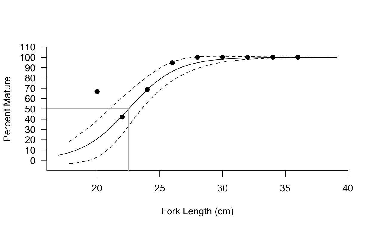
plot(lbins.l50ca$bin,lbins.l50ca$b.p,pch=19,cex.axis=1.0, cex=1.0,cex.lab=1.0, bty="l",xlab="Fork Length (cm)",ylab="Percent Mature"
     ,ylim=c(-0.1,1.1),yaxt="n",yaxs="i",xaxs="i", xlim=c(16,40))
axis(2,at=c(seq(0,1.1,by=.1)),labels=c(seq(0,110,by=10)), cex.lab=1.0,cex.axis=1.0, las=1)
curve((exp(coef(glm.l50ca)[1]+coef(glm.l50ca)[2]*x))/(1+exp(coef(glm.l50ca)[1]+coef(glm.l50ca)[2]*x)),add=T)
lines(l50.cica[,3],l50.cica[,1],lty=2)
lines(l50.cica[,3],l50.cica[,2],lty=2)
lines(c(l50ca,l50ca),c(-0.1,.5), lwd=2,col="grey",lty=1, font=2)
lines(c(16,l50ca),c(.5,.5), lwd=2,col="grey",lty=1,font=2)